Gradient and stochastic gradient descent
Table of Contents
Iterative methods — overview
In these algorithms, we hope to find a value of \(w\) such that a loss function \(f\) is minimized. The algorithms are of the form \(w_{k+1} = w_k + t_k d_k\) where \(d_k\) is some vector and \(t_k\) is a positive number referred to as the "step size."
Recall that the gradient \(\nabla f(w_k)\) points in the direction of steepest increase of a surface at the point \(w_k\). If we are minimizing a loss function, we would like vector \(d_k\) to be in a decreasing direction, namely, the angle between \(d_k\) and \(\nabla f(w_k)\) should be between 90 and 270 degrees. That holds iff \(\cos(\theta) \leq 0\), i.e.
Thus \(d_k\) is a descent direction iff \(\inner{d_k}{\nabla f(w_k)} \in [\norm{d_k}\norm{\nabla f(w_k)}, 0)\).
Note that the direction of steepest decrease would be \(-\nabla f(w_k)\). This choice gives us "the gradient method" (Fawzi, 2023a, Lecture 4).
Using a constant step size may cause us to not converge or converge slowly (see Murphy, 2022, p. 284-285 for examples). The step size can be chosen at each step point \(k\) in an adaptive manner. This will be covered below.
Some ways of evaluating convergence
These are from Royer, 2024. This is not an exhaustive list, as even the results below have different forms than the three listed here.
(1) \(\norm{w_k - w^\ast} \to 0\) as \(k \to \infty\)
Comment: even if we don't know the value of \(w^\ast\) in advance, under certain assumptions we can guarantee this convergence.
(2) \(f(w_k) \to f^\ast\) as \(k \to \infty\)
Same comment as for (1) applies.
(3) \(\norm{\nabla f(w_k)} \to 0\) as \(k \to \infty\)
Note that \(\nabla f(w_k) \to 0\) as \(k \to \infty\) iff \(\norm{\nabla f(w_k)} \to 0\) as \(k \to \infty\), so this is saying that the first order necessary condition is getting closer and closer to being satisfied. Unfortunately since the condition is not a sufficient condition, (3) does not give us a guarantee of convergence on its own.
The gradient method
For a function \(f\), we calculate \(w_{k+1} = w_k - t_k \nabla f(w_k)\).
Assume \(f\) is \(L\)-smooth (see L-smoothness and strong convexity).
We will show results for three types of functions: non-convex functions, convex functions, and strongly convex functions.
Non-convex functions
Theorem: Let \(f\) be \(L\)-smooth, and let \(k\) be an arbitrary step. If \(t_k \in (0, 2/L)\), then \(f(w_{k+1}) < f(w_k)\).
(Royer, 2024, p. 23, Proposition 2.11)
Proof:
This proof is directly from Royer, 2024, p. 23.
Since \(f\) is \(L\)-smooth,
If \(-t_k + (L/2) t_k^2 < 0 \quad (\iff t_k < 2/L)\), then \(f(w_k - t_k \nabla f(w_k)) < f(w_k)\).
\(\square\)
We now show another Lemma that relates to method (3) for measuring convergence.
Theorem: Let \(f\) be \(L\)-smooth, and let \(k\) be an arbitrary step. If \(t_k = 1/L\), then
(Royer, 2024, p. 23)
Proof:
This is from Royer, 2024, with my additions.
Setting \(t_k = 1/L\) and using the inequality from above gives
and therefore
Subtracting duplicate terms from both sides gives
Using the \(f_{\text{low}}\) assumption, we have
[Claim: we show that \(\min\{a_1^2, \ldots, a_K^2\} = (\min\{a_1, \ldots, a_K\})^2\).
Define \(f: [K] \to \{a_1, \ldots, a_K\}\) by \(f(k) = a_k\) for all \(k \in [K]\). Recall that for \(a \geq 0, b \geq 0\), \(a < b \iff a^2 < b^2\) (Bartle & Sherbert, 2011). Thus for \(f \geq 0\), \(f(i) < f(j) \iff f(i)^2 < f(j)^2\).
This implies that \(\argmin_k \{f(k)\} = \argmin_k \{f(k)^2\}\).
We now show that \(\min_k f(k)^2 = (\min_k f(k))^2\):
so the claim is proved.]
By the claim, we have
\(\square\)
Convex functions
Theorem: If \(f\) is convex and \(L\)-smooth w.r.t. the Euclidean norm, with a constant step-size \(t_k = t \in (0, 1/L]\), then
or achieving accuracy \(\varepsilon\) takes
steps.
We can also say convergence is on the order \(O(1/k)\).
(Fawzi, 2023a)
Proof: Fawzi, 2023a.
Strongly convex functions
Theorem: If \(f\) is \(m\)-strongly convex and has \(L\)-Lipschitz continuous gradient w.r.t the Euclidean norm and \(t = 2 / (m + L)\), then
where \(\kappa = L / m \geq 1\). Achieving accuracy \(\varepsilon\) more than a constant times \(\log(1/\varepsilon)\) steps. We can also say convergence is of the order \(O(\gamma^k)\) where \(\gamma \in (0, 1)\).
(Fawzi, 2023a)
Proof: Fawzi, 2023a.
Note on convergence speed
We observe that for \(\gamma \in (0, 1)\), \(\gamma^k\) converges faster than \(1/k\). In fact, \(\gamma^k = o(k^{-a})\) for any \(a \in \mb{Z}_{+}\). Using the fact that both \(\gamma^k\) and \(k^{-a}\) approach 0 in the limit, we use l'Hopital's rule:
Step size
Generally, we don't know the "best" choice of step size. This is one method for finding the largest step size that still satisfies the condition for decrease in the Theorem above:
Backtracking line search (ref. Fawzi, 2023a;, Murphy 2022): starting from a large enough value of \(t_k \leftarrow \widehat{t_k}\) we decrease \(t_k \leftarrow \beta t_k\) (for some \(\beta \in (0, 1)\)) until we have
is satisfied.
Second-order methods
First-order methods do not use the curvature of the parameter space. One method which does is Newton's method (Fawzi, 2023b; Fawzi, 2023c):
Recall the Taylor formula up to second order:
If we ignore the \(o(\norm{h}^2)\) term, the right-hand side is an approximation of the value of \(f(w + h)\) based on the value of \(f\) at \(w\). We wish to find an \(h\) that minimizes \(f(w_k + h)\); we use this approximation to do so, and the resulting \(w_k + h\) will be \(w_{k+1}\).
If we minimize the right-hand side with respect to \(h\), we get \(h = -(\nabla^2 f(w))^{-1} \nabla f(w)\):
[Letting \(g(x) = x^T Ax\),
so \((\partial g(x) / \partial x) = x^T(A + A^T)\) (Edelman & Johnson, 2023).
Now letting \(g(x) = x^T v\) where \(v\) is a vector,
so \((\partial g(x) / \partial x) = v^T\).
Using the above,
so \(h = -(\nabla^2 f(w))^{-1} \nabla f(w)\).]
Thus we set \(w_{k+1} = w_k -(\nabla^2 f(w_k))^{-1} \nabla f(w_k)\).
Theorem: For \(f \in \mc{C}_{L}^{2,2}(\mb{R}^d)\) where \(f\) is \(m\)-strongly convex, Newton's method has quadratic convergence:
(Fawzi, 2023b, Lecture 15) (see same reference for Proof)
Defining \(r_k = (M / 2m^2) \norm{\nabla f(w_k)}\), we have \(r_{k+1} \leq r_k^2\), so \(r_k \leq r_0^{2^k}\). In particular, if \(r_0 < 1\), we will have \(r_k \to 0\) as \(k \to \infty\).
This leads to (Fawzi, Lecture 15):
thus \(f(w_k) - f^\ast \leq r_0^{2^k}\). We conclude that if \(f\) is \(m\)-strongly convex and if an \(w_0\) can be found such that \(r_0 < 1\), we will have convergence on the order of \(O(\gamma^{2^k})\).
Note that a modified version of Newton's method (called just "Newton's method" by Murphy, 2022) adds a step size: \(w_{k+1} = w_k - t_k {\nabla^2 f(w_k)}^{-1} \nabla f(w_k)\).
Momentum
Polyak's momentum
"Gradient descent can move very slowly along flat regions of the loss landscape" (Murphy, 2022, p. 287).
This can be addressed by including an additional term to the gradient term; this is called Polyak's momentum method. The word "momentum" here refers to the fact that our base value is no longer \(w_k\) but \(w_k\) plus the "momentum" we had from going from \(w_{k-1}\) to \(w_k\).
(Chen, 2023)
(Note that if \(\beta = 0\) we just have the gradient method.)
Nesterov momentum
"One problem with the standard momentum method is that it may not slow down enough at the bottom of a valley, causing oscillation" (Murphy, 2022, p. 288). Nesterov momentum can address this.
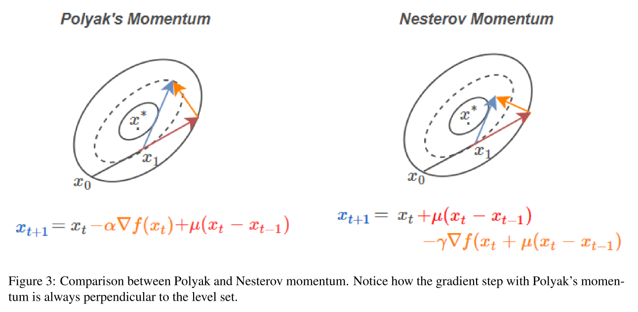
(Image and caption from Mitliagkas, 2018, p. 3)
Stochastic gradient descent (SGD)
For the analyses in this section to work, it must be the case that we are minimizing a sum of functions, namely that we minimize \(f(w) = \sum_{i=1}^n f_i(w)\). This fits with minimizing empirical risk (the estimator of theoretical risk; we assume our data is i.i.d. in this framework):
for a loss function \(\ell\).
For stochastic gradient descent, we can only state our performance guarantees in terms of expectation, where expectation is taken over the random variable used to sample the subset of gradients chosen.
Under SGD, our update is: \(w_{k+1} = w_k - t_k \nabla_w f_{I_k}(w_k)\), where \(I_k \sim \text{Multinoulli}(n, 1/n, \ldots, 1/n)\) (i.e. a discrete random variable taking values in \(\{1, \ldots, n\}\), with each of these values having probability \(1/n\)). The gradient used at step \(k\) is thus a random variable \(\nabla f_{I_k}(w_k)\) with realized value \(\nabla f_{i_k}(w_k)\). Also, \(w_{k+1}\) and thus \(f(w_{k+1})\) is a function of the random variable \(I_k\).
Defining the trace variance
Let \(X\) be a random vector and let \(f(X) = (f_1(X), \ldots, f_n(X))\). I define the "trace Variance" as \(\text{trVar}_X[f(X)] = \text{E}_X\left[\norm{f(X) - E_X[f(X)]}^2\right]\). Observe that
Also note that
where the last step is by using the fact that the inner product is a sum and applying the expectation operator.
This property is similar to the behavior of the variance operator for scalar-valued functions of random variables.
We will first apply the trace variance to the quantity \(g(I_k) = \nabla f_{I_k}(w_k)\) where \(g\) is our function of the random variable \(I_k\), where \(I_k\) is a Multinoulli as above.
Finding a potential decrease in \(E_{I_k}[f(w_{k+1})]\)
Lemma: Let \(f\) be \(L\)-smooth. Assume there exists \(\sigma^2 > 0\) such that \(\trVar_{I_k}[\nabla f_{I_k}(w_k)] \leq \sigma^2\). Then
(Royer, 2023, p. 14, Proposition 2.3.2)
Proof:
We will roughly follow the argument of Royer, 2023, p. 13 - 14, but with clarifying statements and a new definition added, which results in Assumption 2.3.2 (2) not being needed in our proof.
Assume \(f\) is \(L\)-smooth. We attempt to bound \(f(w_{k+1})\) by a Taylor expansion at \(w_k\) (the gradients are all taken with respect to \(w\)):
where the last step is taken by the Lemma from L-smoothness and strong convexity that says \(\inner{\nabla^2 f(x) u}{v} \leq L \norm{u}\norm{v}\).
Take the expectation with respect to \(I_k\):
Observe that
so we have
We now assume there exists a positive \(\sigma^2\) such that \(\trVar_{I_k}[\nabla f_{I_k}(w_k)] \leq \sigma^2\). Note that since \(\E_{I_k}\left[\nabla f_{I_k}(w_k)\right] = \nabla f(w_k)\)
which we could write as
Using this with the above gives
\(\square\)
Depending on the quantities on the right hand side, we may have a decrease in the expected value for an arbitrary step.
Bounding the expectation of \(f(w_k) - f^\ast\) for an \(m\)-strongly convex function
If \(f\) is \(m\)-strongly convex, we will be able to guarantee a type of convergence in expectation. (FIX: Assuming this will guarantee (by Royer, 2023, p. 14, Lemma 2.3.1))
Theorem: Let \(f\) be \(L\)-smooth and \(m\)-strongly convex with \(m \leq L\). Let \(t_k = t \in (0, 1/L]\). Assume there exists \(\sigma^2 > 0\) such that \(\trVar_{I_k}[\nabla f_{I_k}(w_k)] \leq \sigma^2\). Then we have
and thus since \(1 - mt \in (0, 1)\),
(note that the decrease in expectation occurs at rate \(O(\gamma^k)\) where \(\gamma \in (0, 1)\)).
(this is from Royer, 2023, Theorem 2.3.1, but he does not include the last statement involving \(\limsup\).)
Proof:
First, since \(f\) is \(L\)-smooth and \(m\)-strongly convex we have
(Royer, 2023, p. 14, Lemma 2.3.1)
Using this with our inequality gives
Choosing a fixed step-size \(t_k = t \in (0, 1/L]\) gives
so we have
Adding and subtracting \(f^\ast\) to the LHS gives
so that
We note that \(1 - mt \in (0, 1)\) since \(m \leq L \implies t \leq 1/m\) and \(0 \leq t \leq 1/m\) implies \(0 \leq mt \leq 1\), which implies \(1 - mt \in (0, 1)\).
We subtract a term from both sides, giving
We take the expectation of both sides with respect to \(I_{k-1}\):
Continuing until \(\text{E}_1\), and writing \(E_{1 \cdots k}[\bullet] := E_{I_1}[E_{I_2}[\cdots E_{I_k}[\bullet]\cdots ]\), we have
Shifting indices down by one and adding a term to both sides gives
and thus since \(1 - mt \in (0, 1)\),
\(\square\)
It can be shown (Royer, 2023, p. 16-17, Theorem 2.3.2) that for all the same assumptions but using a particular diminishing step size as opposed to a constant step size, we have
for some relevant constants \(\nu, \gamma\) not involving \(k\), i.e. we have convergence with rate \(O(1/k)\).
This is a slower convergence rate than when we use a constant step-size, but we actually converge to the optimal value in expectation rather than to a neighborhood of the optimal value (Royer, 2023, p. 18).
Non-convex case
For stochastic gradient descent with constant step size, we have results that can be used in conjunction with the third of our "convergence" criteria, namely the one which uses the squared norm of the gradient at each step. First, we have
(Royer, 2023, p. 18, Theorem 2.3.3)
where the expectation is again taken over all indices. I.e. the average expected squared norm of the gradients is bounded above by a variance term plus a term that is \(O(1/K)\).
For a sequence of decreasing step sizes satisfying particular assumptions,
(Royer 2023, p. 19, Theorem 2.3.4)
i.e. regardless of \(\sigma^2\), a weighted sum of the expected value of squared norms of gradients converges to 0 as step size goes to infinity.
Mini-batch SGD: a variance reduction technique
Intuition: SGD uses a sample of size one from the full set of gradients \(\{f_i\}\) as an estimate of \(f\). Using the average of a larger sample should reduce the variance of the estimator (in particular, we will show that it minimizes the trace variance of the estimator). In machine learning, at least in this context, a sample is referred to as a "mini-batch." The mini-batch can be drawn with or without replacement; here we assume it is drawn with replacement.
Applying the trace variance to a mini-batch
Let \(S_k = (I_{k,1}, \ldots, I_{k,M})\) where \(M\) is the size of the mini-batch at step \(k\) (the subscript \(k\) is left off of \(M\) for readability), where for each \(m \in [M]\), \(I_{k,m}\) is \(\text{Multinoulli}(n, 1/n, \ldots, 1/n)\) and where for all \(i, j \in [M], i \neq j\) we have that \(I_{k,i}, I_{k,j}\) are pairwise independent.
Let \(V^2\) denote the trace variance of \(f(I_{k,j})\) for arbitrary \(j\). Note that
Thus the trace variance behaves like the variance for an i.i.d sample.
Let \(m_k = (1/M) \sum_{m=1}^M \nabla f_{I_{k,m}}(w_k)\). Applying the trace variance result to an \(L\)-smooth function gives
Therefore
We assume that for all \(m \in [M]\), \(\trVar_{I_{k,m}}[\nabla f_{I_{k,m}}(w_k)] \leq \sigma^2\). By the above property, we have that ,
so \(\E_{S_k}[\norm{m_k}^2] \leq \norm{\E_{s_k}[m_k]}^2 + (1/M) \sigma^2\).
Recall that
which is not reliant on the fact that \(f(w_k)\) is a sum. Thus the above inequality is \(\E_{S_k}[\norm{m_k}^2] \leq \norm{\nabla f(w_k)}^2 + (1/M) \sigma^2\).
Thus we have
Bounding the expectation of \(f(w_k) - f^\ast\) for an \(m\)-strongly convex function
If we assume that \(f\) is \(m\)-strongly convex, with a constant mini-batch size \(n_b\) and fixed step size \(t\), we can follow the line of argument that was followed for stochastic gradient descent to arrive at a similar inequality:
(Royer, 2023, p. 24)
So the rate of convergence is the same, but with a narrower upper bound on the range of convergence due to the change from \(\sigma^2\) to \(\sigma^2 / n_b\).
The following discussion is paraphrased from Royer, 2023, p. 24. For a moment refer to SGD as SGD1 (where the 1 refers to the fact that a sample of gradients of size one is used at each step) and refer to SGD with mini-batch as SGDMB. For comparison purposes, recall the result for SGD1 for a \(m\)-strongly convex function with constant step-size, but use as our step-size \(t / n_b\):
Thus for a particular upper bound on the range of convergence for SGDMB, SGD1 requires more steps to converge in expectation to within that same range. However, the per-step computational cost of SGD1 is less.
References
Bartle, Robert G. and Donald R. Sherbert. (2011). Introduction to real analysis (Fourth ed.). John Wiley & Sons, Inc.
Chen, Yudong. (2023). Lecture 9-10: Accelerated gradient descent [Lecture notes]
Edelman, Alan and Steven G. Johnson. (2023). Matrix Calculus (for Machine Learning and Beyond) [Lecture notes].
Fawzi, Hamza. (2023a). Topics in convex optimization, Lecture 4: Gradient method [Lecture notes].
Fawzi, Hamza. (2023b). Topics in convex optimization, Lecture 15: Newton's method [Lecture notes].
Fawzi, Hamza. (2023c). Topics in convex optimization, Lecture 16: Newton's method (continued) [Lecture notes].
Mitliagkas, Ioannis. (2018). IFT 6085 - Lecture 6: Nesterov’s Accelerated Gradient, Stochastic Gradient Descent [Lecture notes].
Murphy, Kevin P. (2022). Probabilistic Machine Learning: An Introduction. The MIT Press.
Royer, Clément W. (2023). Lecture notes on stochastic gradient methods [Lecture notes].
Royer, Clément W. (2024). Optimization for Machine Learning [Lecture notes].
How to cite this article
Wayman, Eric Alan. (2025). Gradient and stochastic gradient descent. Eric Alan Wayman's technical notes. https://ericwayman.net/notes/gradient-descent-and-sgd/
@misc{wayman2025gradient-descent-and-sgd,
  title={Gradient and stochastic gradient descent},
  author={Wayman, Eric Alan},
  journal={Eric Alan Wayman's technical notes},
  url={https://ericwayman.net/notes/gradient-descent-and-sgd/},
  year={2025}
}