Nonlinear optimization

Dec 22, 2025

Table of Contents

Definitions
Lyusternik's Theorem
- Remark related to the setup of Lyusternik's Theorem
Nonlinear program
Feasible and descent directions
Fritz John Theorem
Notes on the Fritz John result
The sufficiency of the KKT conditions for nonlinear convex programs
References
How to cite this article

Definitions

Cone

Let $C$ be a nonempty subset of a real linear space $X$. The set $C$ is called a cone iff

$$ x \in C, \lambda \geq 0 \implies \lambda x \in C $$

(Jahn, 2007, p. 79, Definition 4.1)

Definition of tangent direction

Let $M$ be a nonempty subset of $\mathbb{R}^n$ and $x \in M$. A vector $d \in \mathbb{R}^n$ is called a /tangent direction/ of $M$ at $x$ iff there exists a sequence $x_n \in M$ converging to $x$ and a nonnegative sequence $\alpha_n$ such that

$$ \lim_{n \to \infty} \alpha_n (x_n - x) = d $$

(Güler, 2010, p. 47, Definition 2.28)

Note that $\alpha_n$ may converge or may not converge.

Narrower definition

$$ \lim_{n \to \infty} \frac{x_n - x}{t_n} = d $$

We now show that the narrower definition implies the definition of tangent direction. Assume the narrower definition holds. Define $\alpha_n = 1 / t_n$ (incidentally, we have $\alpha_n \to \infty$). Then $\lim_{n \to \infty} \alpha_n (x_n - x) = d$, so the definition of tangent direction holds.

Tangent cone

The tangent cone of $M$ at $x$, denoted by $T_M(x)$, is the set of all tangent directions of $M$ at $x$.

Note that the tangent cone is indeed a cone, shown as follows. Let $d \in T_M(x)$. $\lambda d = \lambda \lim_{n \to \infty} \alpha_n (x_n - x) = \lim_{n \to \infty} (\lambda \alpha_n) (x_n - x)$, so the definition is satisfied with the nonnegative sequence $(\lambda \alpha_n)$. Thus $\lambda d \in T_M(x)$.

Note: when the set $S$ is non-convex, $T_S(\overline{x})$ may not contain $S$. See the following figure:

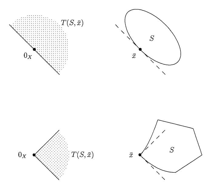
(the above figure is from Jahn, 2007, p. 83)

To see why the set goes outside the cone in the non-convex set, imagine zooming in at the point $\overline{x}$.

Lyusternik's Theorem

Let $f: U \to \mathbb{R}^m$ be a $C^1$ map, where $U \subseteq \mathbb{R}^n$ is an open set. Let $M = f^{-1}(f(x_0))$ be the level set of a point $x_0 \in U$.

If the derivative $Df(x_0)$ is a linear map onto $\mathbb{R}^m$, then the tangent cone of $M$ at $x_0$ is the null space of the linear map $Df(x_0)$, that is,

$$ T_M(x_0) = \{d \in \mathbb{R}^n : Df(x_0) d = 0\} $$

(Güler, 2010, p. 47)

Proof:

$(\subseteq)$

This is what I came up with when trying to follow Güler's proof of this direction (2010, p. 47-48).

Let $d \in T_M(x_0)$.

By the definition of derivative,

$$ f(x_0 + h) = f(x_0) + Df(x_0)(h) + \varphi(h) $$

where

$$ \lim_{h \to 0} \frac{\varphi(h)}{\norm{h}} = 0 $$

Let $(x_n)$ be the sequence from the definition of tangent direction. Letting $h = x_n - x_0$ for a fixed $n$ we have

$$ f(x_n) = f(x_0) + Df(x_0)(x_n - x_0) + \varphi(x_n - x_0) $$

Also recall (see "Little-oh of a sequence" section of Little-oh, the derivative, Taylor's formula) that since $\varphi(h)$ is $o(h)$ as $h \to 0$, it follows that for all sequences $(h_n)$ such that $h_n \to 0$ as $n \to \infty$, we have $\varphi(h_n)$ is $o(h_n)$ as $n \to \infty$. Thus $\varphi(x_n - x_0)$ is $o(x_n - x_0)$ as $n \to \infty$.

Now, since $x_n \in M$, $f(x_n) = f(x_0)$, the above is

$$ 0 = Df(x_0)(x_n - x_0) + \varphi(x_n - x_0) $$

Multiply both sides by the $\alpha_n$ from the definition of tangent direction, so

$$ 0 = Df(x_0) \cdot \alpha_n (x_n - x_0) + \alpha_n \cdot \varphi(x_n - x_0) \quad (\ast) $$

Consider

$$ \alpha_n \cdot \varphi(x_n - x_0) = \frac{\varphi(x_n - x_0)}{\norm{x_n - x_0}} \cdot \alpha_n \norm{x_n - x_0} $$

If the limit as $n \to \infty$ of the right-hand side exists, it equals the product of the limits of each sequence (one a sequence of scalars, one a sequence of vectors, see Lang, 1997, Chapter VII).

Recall that since $\lim_{n \to \infty} \alpha_n (x_n - x_0) = d$, it follows that $\lim_{n \to \infty} \norm{\alpha_n (x_n - x_0)} = \norm{d}$, and also that since $(\alpha_n) \geq 0$, that $\norm{\alpha_n (x_n - x_0)} = \abs{\alpha_n} \norm{x_n - x_0} = \alpha_n \norm{x_n - x_0}$. Thus $\lim_{n \to \infty} \alpha_n \norm{x_n - x_0} = \norm{d} < \infty$.

Therefore

$$ \left(\lim_{n \to \infty} \frac{\varphi(x_n - x_0)}{\norm{x_n - x_0}}\right) \cdot \left(\lim_{n \to \infty} \alpha_n \norm{x_n - x_0}\right) = 0 \cdot \norm{d} = 0 $$

and thus

$$ \lim_{n \to \infty} \alpha_n \cdot \varphi(x_n - x_0) = 0. $$

Thus taking the limit as $n \to \infty$ of both sides of $(\ast)$ gives

$$ 0 = Df(x_0)d + 0 $$

and thus $d \in \text{Ker}(Df(x_0))$.

$(\supseteq)$

This part follows Güler's outline (2010, p. 48) but I filled in details and also used a different approach towards the end.

Let $d \in \text{Ker}(Df(x_0))$. Denote $A = Df(x_0)$. Recall that $Df(x_0)$ is onto $\mathbb{R}^m$. Let $K = \text{Ker}(A)$ and $L = K^\perp$.

By the rank-nullity theorem, $n = \text{dim }\text{Ker}(A) + \text{dim }\text{Im}(A) = \text{dim }\text{Ker}(A) + m$ $\iff \text{dim }\text{Ker}(A) = n - m$. Since $\text{Ker}(A)$ is a subspace of $\mathbb{R}^n$, we can find a basis of $\text{Ker}(A)$, $\{u_1, \ldots, u_{n-m}\}$ and extend it to a basis of $\mathbb{R}^n$, namely $U = \{u_1, \ldots, u_{n-m}, u_{n-m+1}, \ldots, u_n\}$. Note that for $d \in \text{Ker}(A)$,

$$ \begin{align} [d]_U & = a_1 u_1 + \cdots + a_{n-m} u_{n-m} + 0 u_{n-m+1} + \cdots + 0 u_n \notag\\ & = d_1 u^1 + 0 u^2 \notag \end{align} $$

where $d_1 = (a_1, \ldots, a_{n-m})$.

Writing $A$ with respect to this basis and an arbitrary choice of a "to" basis and splitting it into two parts, $A = [D_1 f(y_0, z_0), D_2 f(y_0, z_0)]$. Let $x \in \text{Ker}(A)$.

$$ \begin{align} 0 & = Ax = [D_1 f(y_0, z_0), D_2 f(y_0, z_0)] \begin{bmatrix}d_1 \\0\end{bmatrix} \notag\\ & = D_1 f(y_0, z_0) d_1 \notag \end{align} $$

Since $\text{Ker}(A)$ and $\mathbb{R}^{n-m}$ have the same dimension, they are isomorphic. Therefore for every $x \in \text{Ker}(A)$ there is a vector $(a, 0)$ and vice versa. Thus we could have said: let $a \in \mathbb{R}^{n-m}$ and done the previous calculations in reverse order. Thus for all $a \in \mathbb{R}^{n-m}$ we have $0 = D_1 f(y_0, z_0) a$, which implies $D_1 f(y_0, z_0) = 0$.

Next, we note that since $\text{rank}(A) = m$, $D_1 f(y_0, z_0) = 0$, and $D_2 f(y_0, z_0) \in \mathbb{R}^{m \times m}$, we have that $D_2 f(y_0, z_0)$ is nonsingular.

Recall the first part of the implicit mapping theorem which generalizes the implicit function theorem (Lang, 1997, p. 529): Let $U$ be an open set in $E \times F$, $f: U \to G$ be a $C^p$ map, $(a, b)$ be a point of $U$ with $a \in E$, $b \in F$, and $f(a, b) = 0$. Assume that $D_2 f(a, b): F \to G$ is invertible (as a continuous linear map). Then there exists an open ball $V$ centered at $a$ in $E$ and a continuous map $g: V \to F$ such that $g(a) = b$ and $f(x, g(x)) = 0$ for all $x \in V$. (note that the part quoted here does not require $f \in C^p$, rather, just that $f \in C^1$).

Define the function $\beta(y, z) = f(y, z) - f(y_0, z_0)$, so $\beta(y_0, z_0) = 0$. Applying the theorem to $\beta$, we can write $\beta(y, g(y)) = 0$ for all $y$ in an open ball $V$ around $y_0$. Taking the derivative with respect to $y$ gives

$$ 0 = \frac{\partial}{\partial y} \beta(y, g(y)) = D_1 \beta(y, g(y)) + D_2 \beta(y, g(y)) Dg(y) $$

At $x_0 = (y_0, z_0)$, certainly

$$ 0 = D_1 \beta(y_0, g(y_0)) + D_2 \beta(y_0, g(y_0)) Dg(y_0) $$

From above, we have $D_1 \beta(y_0, g(y_0)) = 0$, and since $D_2 \beta(y_0, g(y_0))$ is invertible, we have $0 = Dg(y_0)$.

Observing that the above arguments regarding $Df$ hold for $D\beta$ as well since the constant makes no difference, we apply the Theorem to the function $\beta$. Let $(t_n)$ be a sequence such that $t_n \to 0$ as $n \to \infty$. Let $\varepsilon > 0$ be the $\varepsilon$ corresponding to $B_\varepsilon(y_0, z_0) = V$. Define $y_n = y_0 + t_n d_1$. Since $\lim_{n \to \infty} t_n = 0$, there exists $N \in \mathbb{N}$ such that for all $n \geq N$, $y_n \in V$. By the Theorem, for all $n \geq N$ we have that $(y_n, z_n) = (y_n, g(y_n))$ where $\beta(y_n, g(y_n)) = 0$.

Observe that $\beta(y_n, g(y_n)) = 0 \iff f(y_n, g(y_n)) = f(y_0, z_0)$, so for all $n \geq N$, $x_n \in M$.

Now note that

$$ \begin{align} g(y_0 + t_n d) & = g(y_0) + Dg(y_0)(t_n d) + \varphi(t_n d) \notag\\ & = g(y_0) + \varphi(t_n d) \notag \end{align} $$

where $\varphi(t_n d)$ is $o(t_n d)$ as $n \to \infty$. Observe that

$$ \begin{align} \frac{x_n - x_0}{t_n} & = \frac{(y_0 + t_n d_1, g(y_0 + t_n d_1)) - (y_0, g(y_0))}{t_n} \notag\\ & = \left(d_1, \frac{g(y_0 + t_n d_1) - g(y_0)}{t_n}\right) \notag\\ & = \left(d_1, \frac{\varphi(t_n d_1)}{t_n}\right) \notag\\ \end{align} $$

and therefore

$$ \lim_{n \to \infty} \frac{x_n - x_0}{t_n} = \lim_{n \to \infty} \left(d_1, \frac{\varphi(t_n d_1)}{t_n}\right) = (d_1, 0) = [d]_U $$

Thus $d \in T_M(x_0)$ and we have shown that $\text{Ker}(Df(x_0)) \subseteq T_M(x_0)$.

$\square$

Remark related to the setup of Lyusternik's Theorem

Claim:

$$ \text{Ker}(Df(x_0)) = \{d \in \mb{R}^n: \inner{\nabla f_i(x_0)}{d} = 0, i \in [m]\} $$

and $Df(x_0)$ is surjective iff $\{\nabla f_i(x_0)\}_{i=1}^m$ are linearly independent.

(this is the "Remark" of Güler, 2010, p.47, i.e. "It is easy to verify that...")

Proof:

(This is my proof which verifies the above.)

For the first statement:

Define $S = \{d \in \mb{R}^n: \inner{\nabla f_i(x_0)}{d} = 0, i \in [m]\}$.

Let $x \in \text{Ker}(Df(x_0)) \equiv Df(x_0)x = 0$

$$ \begin{align*} & \equiv \begin{pmatrix} \frac{\partial f_1}{\partial x_1} & \cdots & \frac{\partial f_1}{\partial x_n} \\ \vdots & & \vdots \\ \frac{\partial f_m}{\partial x_1} & \cdots & \frac{\partial f_m}{\partial x_n} \end{pmatrix} x = 0 \\ & \equiv \begin{pmatrix} \nabla^T f_1(x_0) \\ \vdots \\ \nabla^T f_m(x_0) \end{pmatrix} x = 0 \\ & \equiv \begin{pmatrix} \inner{\nabla f_1(x_0)}{x} \\ \vdots \\ \inner{\nabla f_m(x_0)}{x} \end{pmatrix} = 0 \\ & \equiv x \in S \end{align*} $$

For the second statement, $Df(x_0)$ is surjective iff $\text{dim}(\text{Im } Df(x_0)) = m$, which holds iff the column rank of $Df(x_0)$ equals $m$. Since the column rank of a matrix equals its row rank, this holds iff the rows of $Df(x_0)$ are linearly independent. Finally, the set of transposes of the gradients are linearly independent iff the gradients themselves are. $\square$

Nonlinear program

Definition: A nonlinear program $P$ is a constrained optimization problem having the form

$$ \begin{array}{ll} \min & f(x) \\ \text{s.t.} & \forall i \in [r] \quad g_i(x) \leq 0 \\ & \forall j \in [r] \quad h_j(x) = 0 \end{array} $$

(Güler, 2010, p. 209)

Definition: $I(x) = \{i ; g_i(x) = 0\}$ is the index set of active constraints at $x$.

(Güler, 2010, p. 210)

Feasible and descent directions

This section closely follows Güler, 2010, p. 209-211 and much of it is directly quoted (I filled in the details of the "We will show..." part).

The feasible region of a problem $P$ is defined as

$$ \mc{F}(P) = \{x \in \mb{R}^n : \forall i \enspace g_i(x) \leq 0, \enspace \forall j \enspace h_j(x) = 0\} $$

A point $x^\ast$ is a feasible point iff $x \in \mc{F}(P)$.

For a point $x^\ast \in \mc{F}(P)$, a tangent direction $d$ at $x^\ast$ is called a feasible direction. The set of feasible directions is denoted $\mc{FD}(x^\ast)$.

A vector $d \in \mb{R}^n$ is called a descent direction for $f$ at $x^\ast$ iff $\exists\, (x_n) \quad x_n \to x^\ast$ and $\forall n \quad f(x_n) \leq f(x^\ast)$. If the inequality is strict, then it is called a strict descent direction. The set of strict descent directions is denoted $\mc{SD}(f; x^\ast)$.

We now consider an important Lemma.

Lemma (Güler, page 210) If $x^\ast \in \mc{F}(P)$ is a local minimum of $P$, then $\mc{FD}(x^\ast) \cap \mc{SD}(f; x^\ast) = \emptyset$.

Proof: If the intersection is not empty, then there exists a sequence $(x_n)$ such that for all $n$, $f(x_n) < f(x^\ast)$ in $\mc{F}(P)$, so $x^\ast$ would not be a local minimum, which is a contradiction.

It is sometimes hard to make use of this Lemma, so we define "linearized" versions of the above as follows.

The set of linearized strict descent directions for $f$ at $x^\ast$ is defined as

$$ \mathcal{LSD}(f; x^\ast) := \{d ; \inner{\nabla f(x^\ast)}{d} < 0\}. $$

The set of linearized feasible descent directions for $f$ at $x^\ast$ is defined as

$$ \mathcal{LFD}(x^\ast) := \{d ; \forall\, i \in [r] \enspace \inner{g_i(x^\ast)}{d} < 0, \enspace \forall\, j \in [m] \enspace \inner{h_j(x^\ast)}{d} = 0\}. $$

Lemma: Let $f: U \to \mathbb{R}$ be differentiable on $U \subseteq \mathbb{R}^n$, $U$ open. If $d \in \mathcal{LSD}(x^\ast)$, then for all $x \in U$, for all $t > 0$ such that $t$ is "small enough" (defined precisely below), $f(x^\ast + td) < f(x^\ast)$. If $d \in \mathcal{LFD}(x^\ast)$ and $g_i$ is an active constraint at $x^\ast$, then for all small enough $t > 0$, $g_i(x^\ast + td) < g_i(x^\ast)$.

Proof:

(from Güler, 2010, p. 122)

Let $f: U \to \mathbb{R}$ be differentiable on $U \subseteq \mathbb{R}^n$, $U$ open.

Let $d \in \mathcal{LSD}(f; x^\ast)$. For $\varphi(td)$ where $\lim_{t \to 0} \varphi(td) / t = 0$,

$$ \begin{align} f(x + td) & = f(x) + \inner{\nabla f(x)}{td} + \varphi(td) \notag\\ & = f(x) + t \left[\inner{\nabla f(x)}{d} + \frac{\varphi(td)}{t}\right] \quad (\ast) \notag\\ \end{align} $$

Then, for small enough $t > 0$, since $\inner{\nabla f(x)}{d} < 0$, we have $(\ast) < f(x)$.

[Full argument for this: denoting $g(t) = \varphi(td)/t$, $\lim_{t \to 0} g(t) = 0 \equiv \forall\, \varepsilon > 0 \quad \exists\, \delta > 0 \quad \abs{t} < \delta \implies \abs{g(t)} < \varepsilon$.

Note that $\inner{\nabla f(x)}{d} + g(t) < 0 \iff -\inner{\nabla f(x)}{d} > g(t)$ (and, we have $\inner{\nabla f(x)}{d} < 0$).

So for $\varepsilon = -\inner{\nabla f(x)}{d} \quad \exists\, \delta > 0 \quad g(t) < \varepsilon$.

So for $0 < t < \delta$, we have

$$ t \left[\inner{\nabla f(x)}{d} + g(t)\right] < 0 $$

Thus for "small enough" $t$, $f(x + td) < f(x)$.]

The same argument can be made for the second part: thus for $d \in \mathcal{LFD}(x^\ast)$, $t > 0$ small enough, and $g_i$ active at $x^\ast$, we have $g_i(x^\ast + td) < g_i(x^\ast)$.

$\square$

Fritz John Theorem

Using the above, as well as a result called Motzkin's transportation theorem, we can show the following Theorem:

Theorem (Fritz John): If $x^\ast$ is a local minimizer of $P$ and $f, g_i, h_j$ are continuously differentiable in an open neighborhood of $x^\ast$, then there exist multipliers $(\lambda, \mu) = (\lambda_0, \lambda_1, \ldots, \lambda_r, \mu_1, \ldots, \mu_m)$ not all zero, $\lambda \geq 0$ such that

$$ \begin{align*} & \lambda_0 \nabla f(x^\ast) + \sum_{i=1}^{r} \lambda_i \nabla g_i(x^\ast) + \sum_{j=1}^{m} \mu_i \nabla h_j(x^\ast) = 0, \\ & \forall\, i \in [r] \enspace \lambda_i \geq 0, \enspace \lambda_i g_i(x^\ast) = 0 \end{align*} $$

(Güler, 2010, p. 211)

Proof:

This proof follows Güler (2010, p. 211-212) with me filling in the gaps.

Note that we could rewrite the first equation in the conclusion as

$$ \lambda_0 \nabla f(x^\ast) + \sum_{i \in I(x^\ast)} \lambda_i \nabla g_i(x^\ast) + \sum_{j=1}^{m} \mu_i \nabla h_j(x^\ast) = 0 $$

since if $g_i \not\in I(x^\ast)$, then $\lambda_i g_i(x^\ast) = 0$ implies $\lambda_i = 0$.

Case 1: $\{\nabla h_i(x_0)\}_1^m$ are linearly dependent. Then there exists $\mu = (\mu_1, \ldots, \mu_m) \neq 0$ such that $\sum_{i=1}^m \mu_i \nabla f_i(x_0) = 0$, so setting $\lambda = 0$ we have that the Theorem holds with this $(\lambda, \mu)$.

Case 2: $\{\nabla h_i(x_0)\}_1^m$ are linearly independent.

Let

$$ \begin{align*} S & = \{d ; \inner{\nabla f(x^\ast)}{d} < 0, \inner{\nabla g_i(x^\ast)}{d} < 0, i \in I(x^\ast), \\ & \qquad\qquad \inner{\nabla h_j(x^\ast)}{d} = 0, j \in [m]\} \end{align*} $$

We will use proof by contradiction. Assume $S \neq \emptyset$.

Assume $d \in S$. wlog let $\norm{d} = 1$.

Let $h(x) = (h_1(x), \ldots, h_m(x))$.

$d \in S$ implies $\forall\, j \quad \inner{\nabla h_j(x^\ast)}{d} = 0$, which is equivalent to $Dh(x^\ast) d = 0$ (as in the proof of the "Remark related to setup of Lyusternik's Theorem" above), i.e. $d \in \text{Ker}(Dh(x^\ast))$ .

Recall that the $\nabla h_j(x^\ast)$ are linearly independent iff $Dh(x^\ast)$ is surjective: thus we can apply Lyusternik's Theorem.

Let $M = f^{-1}(f(x^\ast))$. By Lyusternik's Theorem, $d \in \text{Ker}(Dh(x^\ast)) \implies d \in T_M(x^\ast)$, i.e.

$$ \exists\, (\alpha_n) \geq 0 \enspace \exists\, (x_n) \subseteq M \quad x_n \to x^\ast \,\land\, \alpha_n (x_n - x^\ast) \to d $$

Note in particular: since $x^\ast$ is a local minimum, $\forall\, j \in [m] \quad h_j(x^\ast) = 0$, so $h(x^\ast) = 0$.

Since $(x_n) \subseteq M$, $\forall\, n \geq N \quad h(x_n) = 0$.

Consider

$$ \begin{align*} f(x_n) & = f(x^\ast) + \inner{\nabla f(x^\ast)}{x_n - x^\ast} + \varphi(x_n - x^\ast) \\ & = f(x^\ast) + \left[\inner{\nabla f(x^\ast)}{\frac{x_n - x^\ast}{\norm{x_n - x^\ast}}} + \frac{\varphi(x_n - x^\ast)}{\norm{x_n - x^\ast}}\right] \norm{x_n - x^\ast} \\ & = f(x^\ast) + \gamma_n \norm{x_n - x^\ast} \end{align*} $$

where $\varphi(h)$ is $o(h)$ as $h \to 0$, which implies for this $(x_n)$ that $\lim_{n \to \infty} (\varphi(x_n - x^\ast) / \norm{x_n - x^\ast}) = 0$. We have defined the term $\gamma_n$ to be the term in square brackets.

Note that $\alpha (x_n - x^\ast) \to d$ implies $\norm{\alpha_n (x_n - x^\ast)} \to \norm{d}$, so

$$ \frac{x_n - x^\ast}{\norm{x_n - x^\ast}} = \alpha_n (x_n - x^\ast) \cdot \frac{1}{\norm{\alpha_n (x_n - x^\ast)}} \to d \cdot \frac{1}{\norm{d}} = d $$

since $\norm{d} = 1$.

Now, by the continuity of $\inner{\cdot}{\cdot}$,

$$ \begin{align*} \lim_{n \to \infty} \inner{\nabla f(x^\ast)}{\frac{x_n - x^\ast}{\norm{x_n - x^\ast}}} & = \inner{\nabla f(x^\ast)}{\lim_{n \to \infty} \frac{x_n - x^\ast}{\norm{x_n - x^\ast}}} \\ & = \inner{\nabla f(x^\ast)}{d} \end{align*} $$

and therefore we have

$$ \lim_{n \to \infty} \left[\inner{\nabla f(x^\ast)}{\frac{x_n - x^\ast}{\norm{x_n - x^\ast}}} + \frac{\varphi(x_n - x^\ast)}{\norm{x_n - x^\ast}}\right] = \inner{\nabla f(x^\ast)}{d} + 0 $$

Thus in the definition of limit,

$$ \forall\, n \geq N_1 \quad \left|\inner{\nabla f(x^\ast)}{\frac{x_n - x^\ast}{\norm{x_n - x^\ast}}} + \frac{\varphi(x_n - x^\ast)}{\norm{x_n - x^\ast}} - \inner{\nabla f(x^\ast)}{d}\right| < \varepsilon_1 $$

which is equivalent to $\forall\, n \geq N_1$

$$ -\varepsilon_1 + \inner{\nabla f(x^\ast)}{d} \leq \inner{\nabla f(x^\ast)}{\frac{x_n - x^\ast}{\norm{x_n - x^\ast}}} \leq \varepsilon_1 + \inner{\nabla f(x^\ast)}{d} $$

Denote $\inner{\nabla f(x^\ast)}{d} = -\beta$ where $\beta > 0$.

Also for the limit as $n \to \infty$ of the fractional term, we have $\forall n \geq N_2$

$$ -\varepsilon_2 \leq \frac{\varphi(x_n - x^\ast)}{\norm{x_n - x^\ast}} \leq \varepsilon_2 $$

We would like to show that $\gamma_n < 0$. For all $n \geq \max(N_1, N_2)$, we have $T \leq \varepsilon_1 - \beta + \varepsilon_2 \stackrel{\text{want}}{<} 0 \quad (\iff \varepsilon_1 + \varepsilon_2 < \beta)$

So if we choose $\varepsilon_1, \varepsilon_2$ such that $\varepsilon_1 + \varepsilon_2 < \beta$, then $\gamma_n < 0$.

Thus for large enough $n$, $f(x_n) < f(x^\ast)$, contradicting the assumption that $x^\ast$ is a local minimizer. Therefore $S = \emptyset$.

We now invoke Motzkin's transportation theorem, which is quoted in square brackets

[Motzkin's Transporation Theorem: Let $\{a_i\}_1^l$, $\{b_j\}_1^m$, and $\{c_k\}_1^p$ be vectors in $\mb{R}^p$. Then the linear system

$$ \begin{array}{ll} \inner{a_i}{x} < 0 & i \in [l] \\ \inner{b_j}{x} \leq 0 & j \in [m] \\ \inner{c_k}{x} = 0 & k \in [p] \end{array} $$

is inconsistent if and only if there exist vectors (multipliers)

$$ \begin{array}{l} \lambda := (\lambda_1, \ldots, \lambda_l) \geq 0, \lambda \neq 0 \\ \mu := (\mu_1, \ldots, \mu_m) \geq 0 \\ \delta := (\delta_1, \ldots, \delta_p) \end{array} $$

such that

$$ \sum_1^l \lambda_i a_i + \sum_1^m \mu_j b_j + \sum_1^p \delta_k c_k = 0. $$

(Güler, 2010, p. 72-73)]

Considering the system of equations given by the conditions of the set $S$, since the system of equations is inconsistent (since $S = \emptyset$), the multipliers exist.

$\square$

Notes on the Fritz John result

This section reproduces arguments from Güler, 2010, p.212-213.

The mathematical expressions in the conclusion of the above theorem are often called "conditions": they are necessary conditions for a local optimium.

$L(x, \lambda, \mu) = \lambda_0 \nabla f(x) + \sum_{i=1}^{r} \lambda_i \nabla g_i(x) + \sum_{j=1}^{m} \mu_i \nabla h_j(x)$ is called the weak Lagrangian function for $P$ (where $P$ is the programming problem "minimize $f$ subject to the various conditions").

The conditions

$$ \forall\, i \in [r] \enspace \lambda_i \geq 0, \enspace \lambda_i g_i(x^\ast) = 0 $$

are called "complimentary conditions" since for each $i$ we must either have $\lambda_i \geq 0$ or $g_i(x^\ast) \leq 0$ or both.

If $\lambda_0$ we can assume wlog that $\lambda_0 = 1$ and we call $L(x, \lambda, \mu) = \nabla f(x) + \sum_{i=1}^{r} \lambda_i \nabla g_i(x) + \sum_{j=1}^{m} \mu_i \nabla h_j(x)$ the Lagrangian function for $P$.

It would be strange if $\lambda_0$ were 0, since $f$ itself would not appear in the result of the theorem (conditions for optimality).

At an optimal argument (local minimizer) $x^\ast$, we can make an additional assumption (called a "constraint qualification" that results in $\lambda_0 > 0$ and

$$ (1) \quad \begin{cases} \nabla f(x^\ast) + \sum_{i=1}^{r} \lambda_i \nabla g_i(x^\ast) + \sum_{j=1}^{m} \mu_i \nabla h_j(x^\ast) = 0, \\ \forall\, i \in [r] \enspace \lambda_i \geq 0, \enspace \lambda_i g_i(x^\ast) = 0 \end{cases} $$

$(1)$ are called the KKT conditions (they are the same as the Fritz-John conditions but without $\lambda_0$ appearing).

One constraint qualification is $\{\nabla g_i(x^\ast), i \in I(x^\ast), \nabla h_j(x^\ast), j \in [m]\}$ are linearly independent. Another one is Slater's condition:

Definition: A point $x$ satisfies Slater's condition iff $x$ is an optimal argument of $f$, $x \in \mc{F}(P)$, and there exists $x_0 \in \mc{F}(P)$ such that $\forall i \in I(x) \quad g_i(x_0) < 0$.

Corollary (Güler, page 220): If $\{g_i\}$ are convex and $\{h_j\}$ are affine and Slater's condition is satisfied at $x^\ast$, then the KKT conditions are satisfied at $x^\ast$.

Proof: Güler, 2010, p. 220.

Also see Duality theory for another place where Slater's condition is used.

The sufficiency of the KKT conditions for nonlinear convex programs

A nonlinear program $P$ is a nonlinear convex program iff $f$ and $g_i$ are convex, $h$ is affine, and $C \subseteq \mb{R}^n$ is a nonempty convex set (Güler, 2010, p. 281).

Theorem (sufficiency of the KKT conditions for nonlinear convex programs): For a nonlinear convex program $P$, if the KKT conditions hold at a point $x$, then $x$ is an optimal argument of $f$ (and indeed it is globally optimal due to the convexity). (Andréassan, 2020, p. 150, Theorem 5.49).

Proof: See Andréassan, 2020.

References

Andréasson, Niclas, Anton Evgrafov and Michael Patriksson. (2020). An Introduction to Continuous Optimization: Foundations and Fundamental Algorithms (Third ed.). Dover Publications.

Güler, Osman. (2010). Foundations of optimization. Springer Science+Business Media, Inc.

Jahn, Johannes. (2007). Introduction to the theory of nonlinear optimization (Third ed.). Springer Berlin Heidelberg New York.

Lang, Serge. (1997). Undergraduate analysis (Second ed.). Springer Science+Business Media, Inc.

How to cite this article

Wayman, Eric Alan. (2025). Nonlinear optimization. Eric Alan Wayman's technical notes. https://ericwayman.net/notes/nonlinear-optimization/

@misc{wayman2025nonlinear-optimization,
  title={Nonlinear optimization},
  author={Wayman, Eric Alan},
  journal={Eric Alan Wayman's technical notes},
  url={https://ericwayman.net/notes/nonlinear-optimization/},
  year={2025}
}